A practical guide to principal component analysis

Author

jrose

Published

November 27, 2023

The following is a short primer I made for the IBS519 course at Emory in the Fall of 2023 to introduce first-year bioscience students to PCA for use in their research

Part 1: PCA Background

I wanna be the very best…

At the beginning of this course we learned how simple data visualization can help to uncover broader structures within data by plotting relationships between individual variables (or features) one at a time.

Now we are going to to VERY QUICKLY cover another technique that is commonly used to find structure in large, complex, multi-variable datasets:

Principal component analysis

Load Data

To do so let’s bring back our friends….the Pokemon…and all of their stats to see if we can make any new conclusions about them using PCA.

library(tidyverse)

poke = read_csv("./DataSets/pokemon.csv")

Principal component analysis is a dimensional reduction technique that creates NEW variables (principal components) which:

Are not correlated with each other
Try to capture as much of the variance of the data as possible

PCA is often useful when you have LOTS of variables, some of which may be correlated with each other, and where interpretation of each variable/feature individually would take too much time.

Prepare Data

The following is required to successfully perform PCA:

Data must be numeric (no discrete or categorical data)
Each variable should be on the same scale and ideally centered at 0
Must not contain NA values

Let’s walk through preparing our data for each of these criteria:

poke_num <- poke %>% select_if(is.numeric) %>% 
  select(-Number) %>% #Num is just an index variable so we don't want to use it
  mutate(Name=poke$Name)
#^Select numeric values only

poke_num <- drop_na(poke_num) %>%
  column_to_rownames(var="Name")
#^Remove NAs & set rownames to pokemon Name

poke_num_scale <- apply(poke_num, 2, scale) %>% data.frame()
#^Transform our data to scale and center

rownames(poke_num_scale) <- rownames(poke_num)
#^Fix rownames

head(poke_num_scale)

                 Total         HP     Attack    Defense Special.Atk Special.Def
Bulbasaur  -0.86464383 -0.8650069 -0.8562420 -0.6765372 -0.01480364 -0.04587956
Ivysaur     0.01702662 -0.2751045 -0.3932530 -0.1801456  0.55493009  0.55628964
Venusaur    1.23312378  0.5114319  0.3190376  0.5289851  1.31457507  1.35918191
Charmander -0.95585111 -1.1009678 -0.7493984 -0.8892764 -0.20471488 -0.64804876
Charmeleon  0.01702662 -0.3537582 -0.3220240 -0.3574283  0.55493009 -0.04587956
Charizard   1.32433107  0.4327782  0.3902667  0.3517024  1.65641531  0.75701271
                 Speed Generation  Pr_Male    Height_m  Weight_kg Catch_Rate
Bulbasaur  -0.70370909  -1.371074 1.608363 -0.38910342 -0.6078938 -0.8343086
Ivysaur    -0.13830696  -1.371074 1.608363 -0.08879898 -0.5121877 -0.8343086
Venusaur    0.61556254  -1.371074 1.608363  1.00516717  0.8528015 -0.8343086
Charmander  0.05016042  -1.371074 1.608363 -0.49635500 -0.5827905 -0.8343086
Charmeleon  0.61556254  -1.371074 1.608363  0.01845260 -0.4180505 -0.8343086
Charizard   1.36943205  -1.371074 1.608363  0.67268726  0.7037510 -0.8343086

summary(poke$HP)

   Min. 1st Qu.  Median    Mean 3rd Qu.    Max. 
   1.00   50.00   65.00   68.38   80.00  255.00

summary(poke$Attack)

   Min. 1st Qu.  Median    Mean 3rd Qu.    Max. 
   5.00   53.00   74.00   75.01   95.00  165.00

summary(poke_num_scale$HP)

    Min.  1st Qu.   Median     Mean  3rd Qu.     Max. 
-2.24145 -0.66837 -0.07847  0.00000  0.44261  7.39363

summary(poke_num_scale$Attack)

   Min. 1st Qu.  Median    Mean 3rd Qu.    Max. 
-2.4233 -0.7494 -0.1083  0.0000  0.6040  3.2750

Notice how both variables (HP & Attack) now have a mean centered at 0 and relatively similar ranges/scales

Perform PCA & Visualize

Now our data is prepared for PCA. There are many different functions that have been created to help perform PCA in R, each with slightly different attributes. Try asking your favorite GPT model/chatbot to list out all of them sometime.

Today, we will use the princomp() function to do the actual PCA

pca <- princomp(poke_num_scale)

The results of the PCA are now stored in the object named pca. Let’s take a look at what’s inside it.

summary(pca)

Importance of components:
                          Comp.1    Comp.2     Comp.3     Comp.4     Comp.5
Standard deviation     2.1400310 1.2039366 1.06052524 1.02873685 0.96975628
Proportion of Variance 0.3822379 0.1209765 0.09387191 0.08832878 0.07849082
Cumulative Proportion  0.3822379 0.5032144 0.59708631 0.68541509 0.76390591
                           Comp.6     Comp.7     Comp.8    Comp.9    Comp.10
Standard deviation     0.85705152 0.81755855 0.68900108 0.6161671 0.55440766
Proportion of Variance 0.06130664 0.05578679 0.03962173 0.0316877 0.02565382
Cumulative Proportion  0.82521255 0.88099934 0.92062107 0.9523088 0.97796259
                          Comp.11 Comp.12
Standard deviation     0.51384660       0
Proportion of Variance 0.02203741       0
Cumulative Proportion  1.00000000       1

We can also visualize the results. Let’s use a few functions from the “factoextra” package which are designed specifically for visualzing the results of the princomp function.

library(factoextra)
library(patchwork)

p1 <- fviz_pca_ind(pca)
p2 <- fviz_eig(pca)
p3 <- fviz_pca_var(pca)

#fviz_pca_ind(pca, axes=c(2,3))
#fviz_pca_var(pca, axes=c(2,3))

The individual scatter plot shows a scatter plot of the first two PCs for each row in our data (in this case each Pokemon)

p1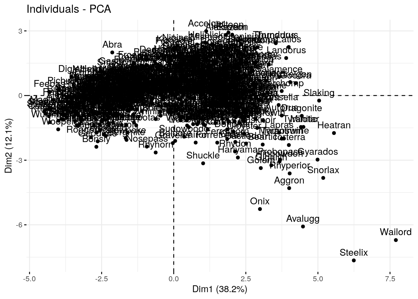

The scree/eigenvector plot shows the percentage of total variance explained by each PC

p1 + p2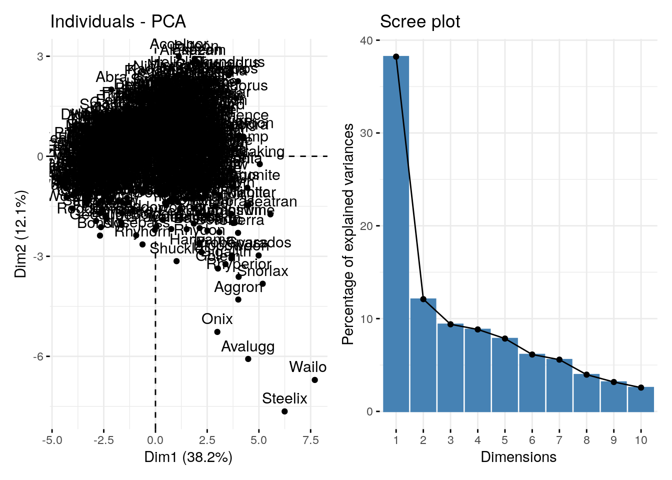

The variable plot shows the “loadings” for each variable in the dataset. The direction of each vector indicates the direction of the variable’s maximum variance, and the length of the vector indicates the strength of the variable’s contribution to the components being plotted.

The angle between any two vectors approximates the correlation between the corresponding variables. A small angle implies a strong positive correlation, an angle around 90 degrees implies little or no correlation, and an angle greater than 90 degrees implies a negative correlation.

p3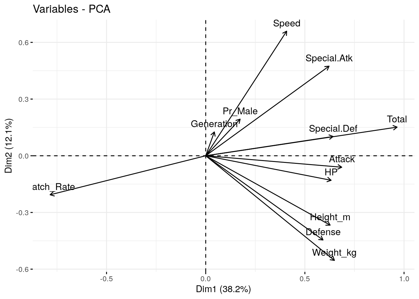

p1 + p3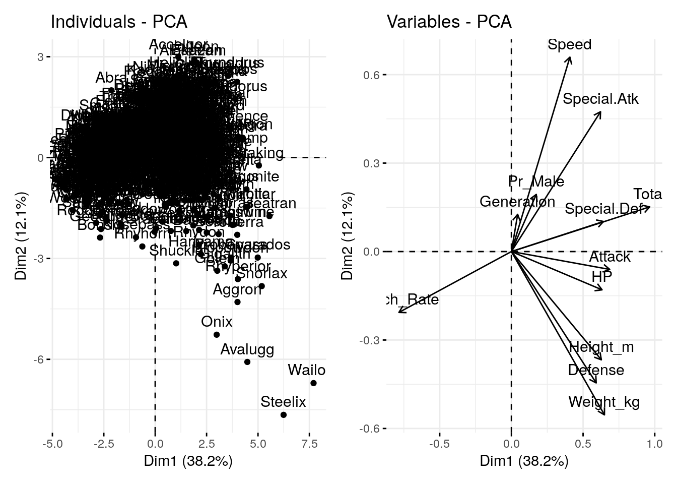

How do the PC results relate to our original data?

To answer this we need to combine our new variables (PCs) with our old data (without the scaling).

A little wrangling to do that:

pca_scores <- pca$scores %>%
  data.frame() %>%
  rownames_to_column(var="Name")


pca_plot <- left_join(pca_scores, poke, by="Name")

And now we can use ggplot to visualize the scatter plot from before, along with the original categorical or numeric data

ggplot(pca_plot, aes(x=Comp.1, y=Comp.2)) + geom_point(aes(color=Catch_Rate)) + scale_color_viridis_c() + theme_minimal()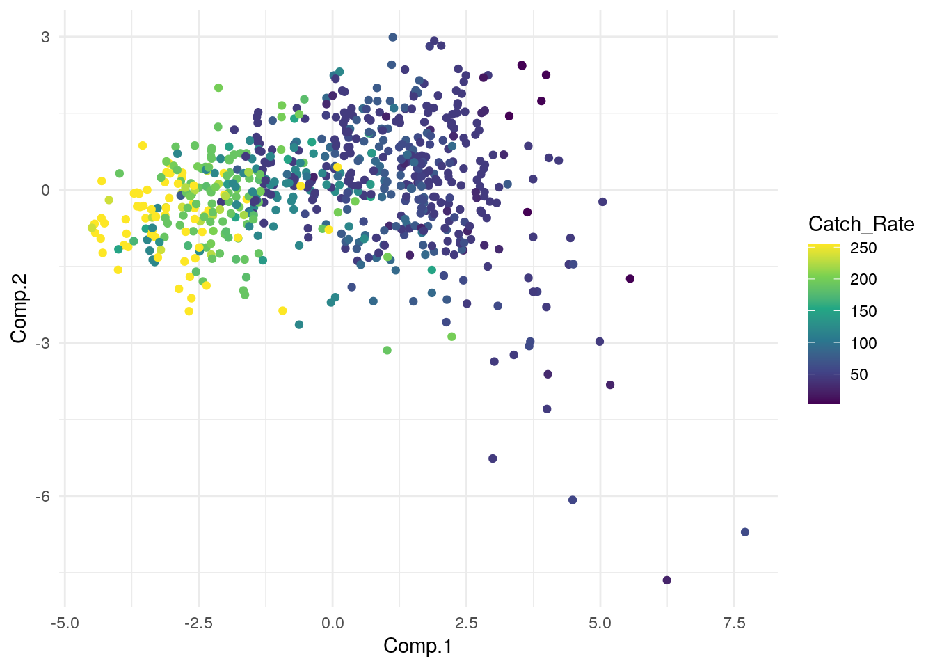

Code

g1 <- ggplot(pca_plot, aes(x=Comp.1, y=Comp.2)) + geom_point(aes(color=Defense)) + scale_color_viridis_c() + theme_minimal()
g2 <- ggplot(pca_plot, aes(x=Comp.1, y=Comp.2)) + geom_point(aes(color=Speed)) + scale_color_viridis_c() + theme_minimal()
g3 <- ggplot(pca_plot, aes(x=Comp.1, y=Comp.2)) + geom_point(aes(color=Weight_kg)) + scale_color_viridis_c() + theme_minimal()

g1 + g2 + g3 + plot_layout(nrow = 2, byrow = FALSE)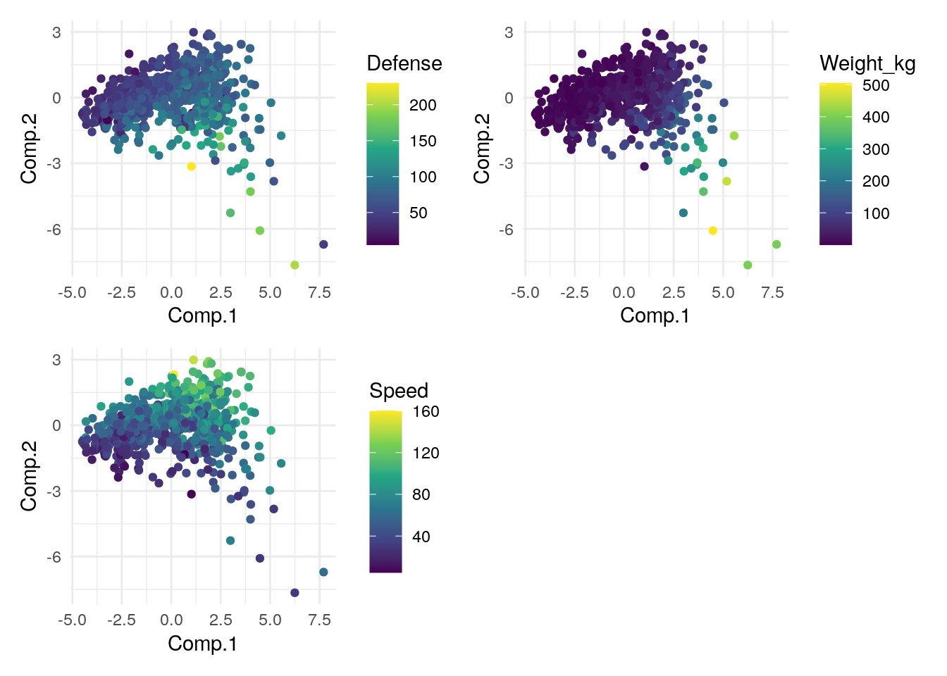

What have we learned about our data from this? Any big observations/conclusions?

Part 2: How PCA can help with modeling

Can we catch ’em all?

The PC variables we create can also be used when creating statistical models…with a few inherent benefits.

Let’s explore this by trying to predict the catch rate variable using other attributes about our pokemon.

Using a traditional variables

reg_model <- glm(Catch_Rate ~ Attack + Defense + Speed + Weight_kg + Height_m + HP + `Special Atk` + `Special Def`, data=pca_plot)
summary(reg_model)


Call:
glm(formula = Catch_Rate ~ Attack + Defense + Speed + Weight_kg + 
    Height_m + HP + `Special Atk` + `Special Def`, data = pca_plot)

Deviance Residuals: 
     Min        1Q    Median        3Q       Max  
-146.674   -24.799     0.986    29.198   181.870  

Coefficients:
               Estimate Std. Error t value Pr(>|t|)    
(Intercept)   327.68172    9.49092  34.526  < 2e-16 ***
Attack         -0.56111    0.09617  -5.835 8.60e-09 ***
Defense        -0.49376    0.09890  -4.992 7.71e-07 ***
Speed          -0.52689    0.09158  -5.754 1.36e-08 ***
Weight_kg       0.04521    0.04756   0.951    0.342    
Height_m       -4.23261    2.96479  -1.428    0.154    
HP             -0.58127    0.09935  -5.851 7.83e-09 ***
`Special Atk`  -0.59105    0.09532  -6.200 1.01e-09 ***
`Special Def`  -0.48401    0.10762  -4.498 8.18e-06 ***
---
Signif. codes:  0 '***' 0.001 '**' 0.01 '*' 0.05 '.' 0.1 ' ' 1

(Dispersion parameter for gaussian family taken to be 2724.921)

    Null deviance: 3602868  on 643  degrees of freedom
Residual deviance: 1730325  on 635  degrees of freedom
AIC: 6932.7

Number of Fisher Scoring iterations: 2

Keep a note of the AIC value here. AIC stands for Akaike Information Criterion which is a measure used in statistics to assess how well a statistical model fits the data.
When comparing models LOWER AIC values are thought to indicate that a model is a relatively better fit for the data.

Using PCs

Now let’s try to do the same using our PCs

PCA_model <- glm(Catch_Rate ~ Comp.1 + Comp.2 + Comp.3 + Comp.4,  data=pca_plot)
summary(PCA_model)


Call:
glm(formula = Catch_Rate ~ Comp.1 + Comp.2 + Comp.3 + Comp.4, 
    data = pca_plot)

Deviance Residuals: 
     Min        1Q    Median        3Q       Max  
-120.709   -24.619     0.719    28.339   147.563  

Coefficients:
            Estimate Std. Error t value Pr(>|t|)    
(Intercept) 107.4519     1.6847  63.783  < 2e-16 ***
Comp.1      -27.4426     0.7872 -34.861  < 2e-16 ***
Comp.2      -12.8318     1.3993  -9.170  < 2e-16 ***
Comp.3        8.9677     1.5885   5.645 2.48e-08 ***
Comp.4        1.6513     1.6376   1.008    0.314    
---
Signif. codes:  0 '***' 0.001 '**' 0.01 '*' 0.05 '.' 0.1 ' ' 1

(Dispersion parameter for gaussian family taken to be 1827.718)

    Null deviance: 3602868  on 643  degrees of freedom
Residual deviance: 1167912  on 639  degrees of freedom
AIC: 6671.5

Number of Fisher Scoring iterations: 2

How do the two models compare ?

Which one would you use?

Potential benefits of using PCA in modeling:

Reducing dimensions of the data makes for a simpler model (less features) which is less likely to overfit data
PCA can be helpful in reducing noise since it retains the most significant principal components and discards the rest
PCA transforms correlated variables into a set of linearly uncorrelated components, which helps to mitigate the issues that arise from multicollinearity.

Take aways

PCA requires clean & numeric data set on roughly the same scale
The princomp() function can be used to perfrom PCA in R. The factoextra package has some good visualization tools designed specifically to work with this function.
Reducing the complexity of models using PCA can help to improve prediction ability

Resources to learn more

This was a very quick, practical guide to using PCA. In the same way that driving a car doesn’t require knowing how internal combustion engines work, you can use PCA without understanding the underlying mechanics. HOWEVER if you do so you better have a mechanic (aka statistician) on hand in case anything breaks down.

If you want to deepen your knowledge and learn more about how PCA works (including the math behind it) check out the following: